Break-Even Graph
Managerial accounting (cost–volume–profit analysis)
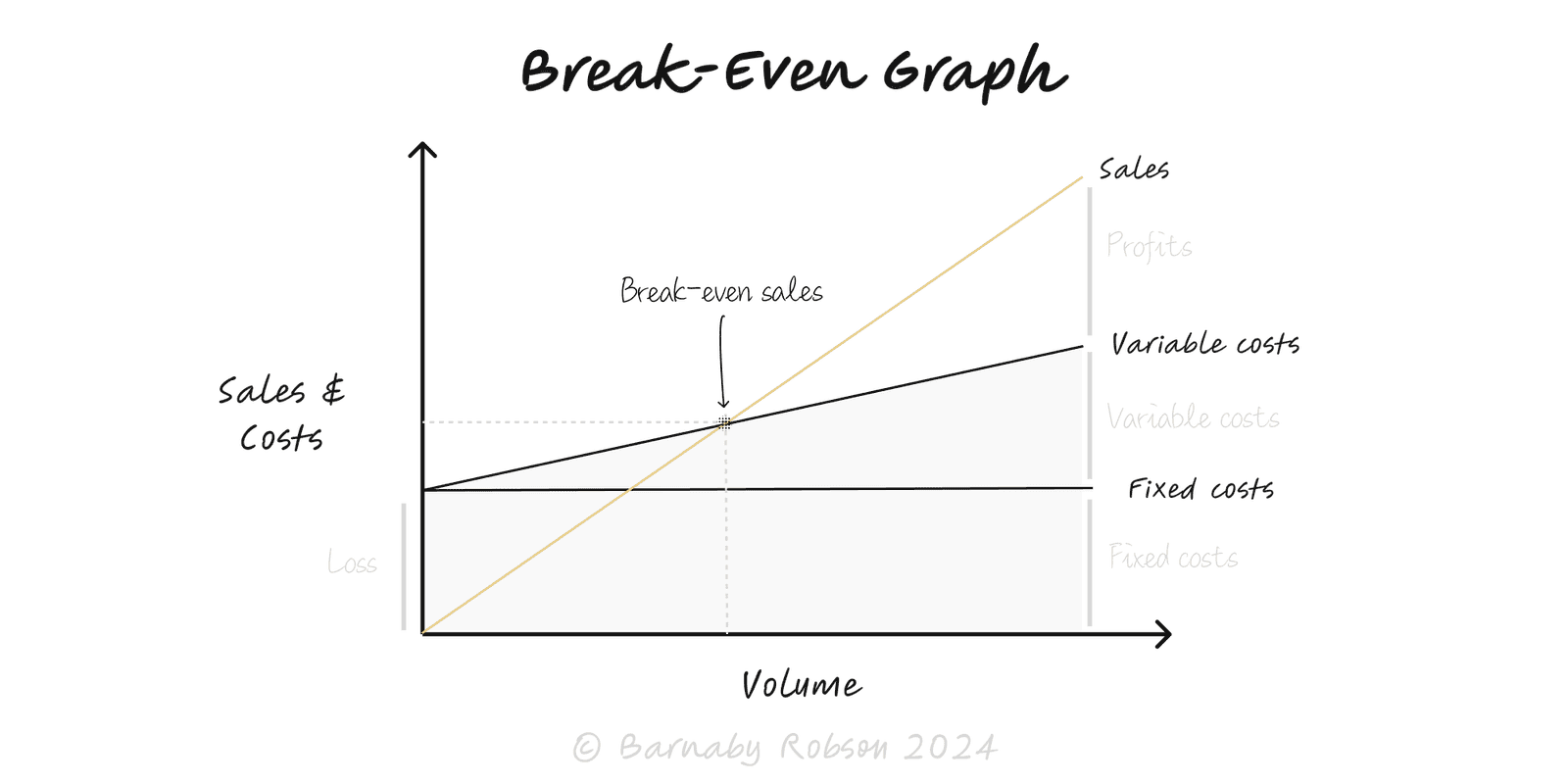
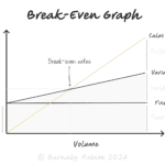
The break-even graph is the classic cost–volume–profit view. It plots total revenue and total cost against units sold. Their intersection is the break-even point (no profit, no loss). With a few inputs you can test prices, cost changes and sales targets, and see how fast profit grows after break-even (operating leverage).
Inputs
- Price per unit (P)
- Variable cost per unit (V)
- Fixed costs (F) – costs that don’t change within the relevant range (rent, salaries, base SaaS, etc.)
Contribution margin: CM = P − V (per unit) and CM% = (P − V) / P.
Break-even units: BE_units = F / (P − V).
Break-even revenue: BE_rev = BE_units × P.
Margin of safety: (Expected sales − BE_units) / Expected sales.
Operating leverage: profit grows faster than revenue once past break-even; sensitivity ≈ Contribution / Operating profit.
Graph: a straight revenue line from the origin with slope P, and a total cost line starting at F with slope V. The crossing is break-even.
Pricing and discount policy – see the volume needed after a price change.
New product / channel – sanity-check unit economics before launch.
Cost-out programmes – estimate how much F or V must fall to reach break-even sooner.
Capacity and sales targets – ensure break-even is reachable within realistic demand.
Subscription/SaaS – adapt to “per-period” units (active subscribers), include churn and CAC payback.
Classify costs – split fixed vs variable within the relevant output range; note any step-fixed costs.
Estimate P and V – include discounts, returns, freight, payment fees; use current mix.
Compute CM, BE_units, BE_rev; add margin of safety against your forecast.
Plot the graph – show revenue and total cost; mark break-even and a few demand scenarios.
Run scenarios – price ±x%, variable cost ±x%, mix shifts, capacity limits; note new BE points.
Decide actions – raise price, change mix, reduce V (supplier, packaging, process), reduce F (leases, tooling), or increase qualified demand.
Review monthly – update with actuals; watch drift in discounts, returns and utilisation.
Misclassifying costs – many “fixed” costs are step-fixed (they jump when capacity is added).
Ignoring mix – multi-product lines need a weighted average CM; mix changes shift break-even.
Leaving out on-costs – shipping, payment fees, commissions, warranty, returns.
SaaS specifics – treat the unit as an active subscriber; incorporate churn and CAC payback (months to recover acquisition cost).
Non-linear realities – price elasticity, capacity ceilings and learning effects bend the straight lines; use the graph as a guide, then model ranges.
Top-line fixation – high volume at low CM can be worse than lower volume at healthy CM%.