Comparative Advantage
David Ricardo (1817)
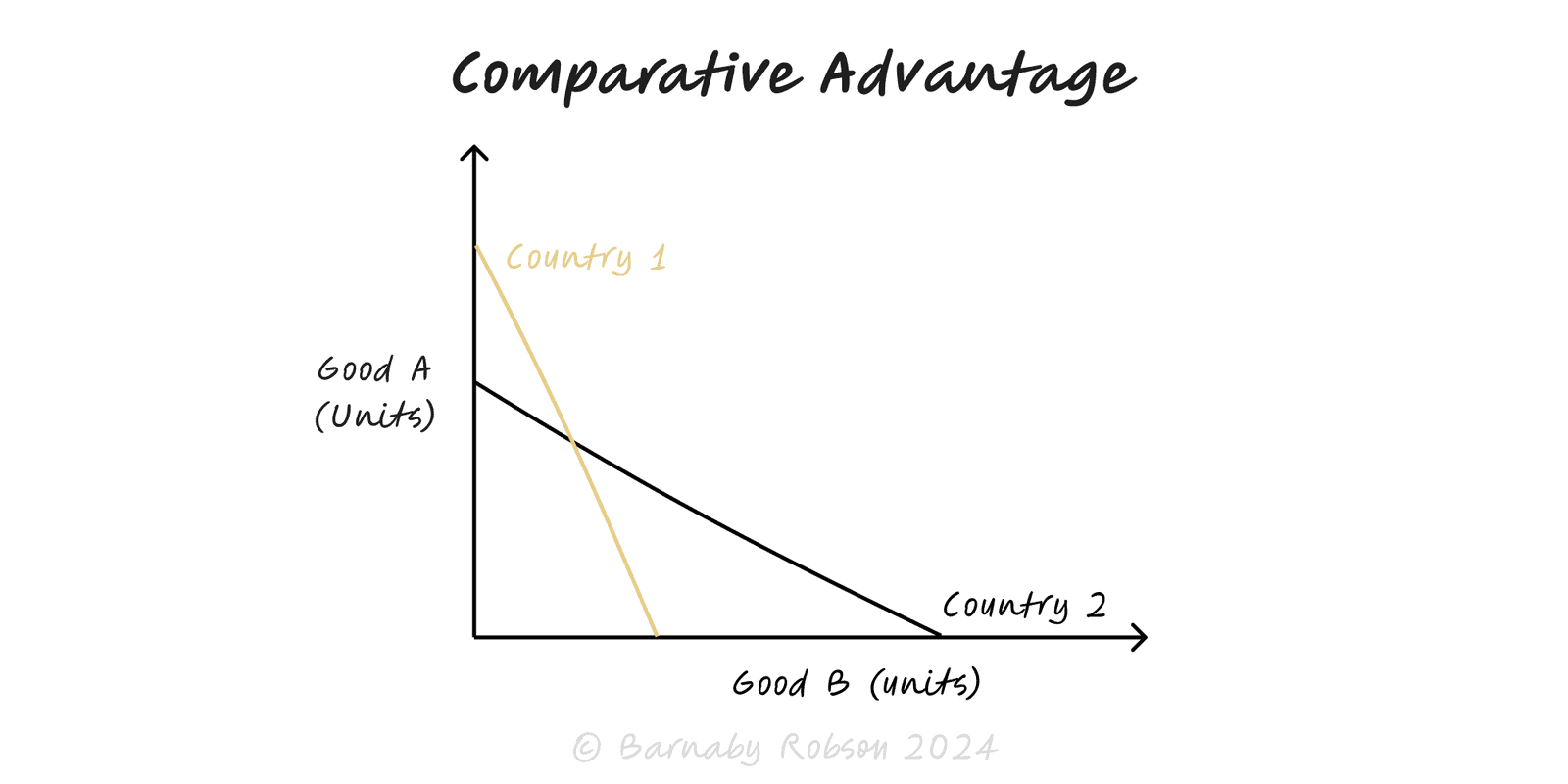
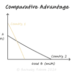
Comparative advantage explains why two parties can both gain from trade even if one is absolutely better at everything. What matters isn’t absolute productivity, but what you give up to make one thing instead of another (opportunity cost). By specialising where your opportunity cost is lowest and trading, total output and joint surplus rise.
Opportunity cost – the value of the best alternative forgone. With two outputs A and B,
• OC(A) = resources for A ÷ resources for B (in units of B), and vice versa.
Comparative vs absolute – you can be slower at both goods (no absolute advantage) yet still have lower OC in one.
Terms of trade – mutually beneficial prices lie between the two parties’ opportunity costs.
Generalises – works for countries, firms, teams and individuals; any context with scarce resources and different trade-offs.
Friction matters – gains must exceed transport, coordination, risk and quality costs.
Sourcing/outsourcing – allocate components to the plant or partner with the lowest opportunity cost, not just lowest wage.
Org design – split work so teams focus on their highest-fit capabilities; partner for the rest.
Personal productivity – delegate tasks where your OC is high (they displace your highest-value work).
Market entry – export where you have a relative edge; import what’s relatively costly for you to produce.
List the outputs (two to start) and the agents (teams/suppliers/countries).
Estimate unit resources (hours, £, capacity points) for each agent × output.
Compute opportunity costs per agent (e.g., OC of Good A = hours(A)/hours(B)).
Assign specialisation – each agent makes the good where its OC is lowest.
Set terms of trade between the two OCs; both sides must be better off than autarky.
Check frictions and risk – transport, defect rate, FX, lead times, IP; include these in the OC.
Pilot and measure – compare delivered cost, cycle time, quality, and resilience; scale if net surplus holds.
Worked mini-example (Ricardo-style)
Hours per unit
• England: Cloth 100h, Wine 120h
• Portugal: Cloth 90h, Wine 80h
Opportunity costs
• England: OC(Cloth) = 100/120 = 0.83 Wine; OC(Wine) = 120/100 = 1.20 Cloth
• Portugal: OC(Cloth) = 90/80 = 1.125 Wine; OC(Wine) = 80/90 = 0.89 Cloth
Specialise
• England → Cloth (lower OC in cloth)
• Portugal → Wine (lower OC in wine)
Terms of trade (example)
• 1 Cloth ↔ 1 Wine (lies between 0.83 and 1.125 Wine per Cloth) benefits both compared with self-sufficiency.
Confusing absolute and comparative advantage – the fastest producer shouldn’t do everything if OC differs.
Ignoring frictions – transport, coordination, defect risk and IP/security can wipe out gains.
Static trap – specialisation can lock you into yesterday’s edge; revisit as tech, scale and learning curves shift.
Capacity & lumpy costs – step-fixed costs or minimum viable scale can break simple ratios.
Unpriced externalities – environmental or geopolitical risks alter true costs.
Single-point dependence – diversify critical inputs; don’t trade resilience for pennies.