Distributions
Probability & statistics (Gauss, Laplace, Pareto, Mandelbrot; modern applied stats)
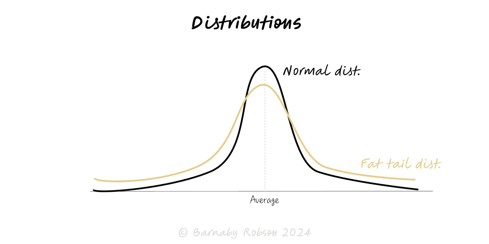
A distribution describes how often values occur. Many business tools assume a normal (Gaussian) bell curve—symmetric, thin-tailed, mean ≈ typical. But lots of real-world phenomena are skewed or heavy-tailed: a few extreme values dominate (sales per product, outages, viral posts, wealth). Picking the right family—normal, lognormal, power-law (Pareto), exponential, Poisson—changes how you summarise, predict and manage risk.
Normal (Gaussian) – additive noise, many small independent effects (CLT). Symmetric, thin tails.
- Heuristics: mean ≈ median; “68–95–99.7%” within 1–2–3σ.
Lognormal – multiplicative growth (price × price × …), non-negative, right-skewed.
- Heuristics: use geometric mean, medians and percentiles; extremes matter.
Exponential – memoryless waiting times between independent events (simple queues, decay).
Poisson – counts of independent rare events per interval (arrivals/defects at low rate).
Power-law (Pareto) – P(X > x) ∝ x^−α above a threshold x_min; few huge values dominate.
- For α ≤ 2 variance is infinite; for α ≤ 1 even the mean diverges (sample averages are unstable).
Mixtures & regime shifts – many domains are blends (e.g., normal body but heavy tail of spikes).
Thin vs heavy tails – thin tails make extremes rare; heavy tails make them decisive.
Risk & reliability – incident sizes, drawdowns, claim severity (heavy tails).
Operations – inter-arrival/wait times (Poisson/exponential), over-dispersion in queues.
Growth/marketing – campaign and creator impacts (lognormal/heavy-tailed).
Finance – returns have fatter tails than normal; stress with percentiles and scenario paths.
Inventory & demand – skewed SKU demand; stock by service levels (quantiles), not averages.
Plot before you model – histogram + log scale versions; compare CDF/CCDF (1−CDF) on log–log for tails.
Summarise robustly – in skew/heavy tails use median, IQR, and percentiles (P90/P95/P99) over mean/σ.
Choose a family
symmetric/thin → normal; strictly positive × multiplicative → lognormal; counts → Poisson/negative binomial; extreme-dominated → Pareto or lognormal tail.
Fit with care – estimate thresholds for tail fits (x_min); check goodness with QQ-plots and hold-outs.
Decide with quantiles – set SLOs, capacity, buffers and risk limits by P95/P99, not average.
Stress the tails – scenario ranges and worst-plausible events; don’t rely on ±2σ if tails are heavy.
Aggregate wisely – sums of heavy-tailed terms stay heavy-tailed; diversification may help less than you expect.
Communicate ranges – show fans/intervals; avoid single-number promises in fat-tail domains.
Assuming normal by habit – in heavy tails, averages understate risk and “six sigma” fails.
Misreading logs – a straight line on log–log suggests a power law only above a threshold; test alternatives (lognormal) before declaring Pareto.
Using σ-based rules on skew – “mean ± 2σ” thresholds break when mean ≠ typical.
Truncation/censoring – caps/hard limits hide tails; correct for it or you’ll be over-confident.
Stationarity assumptions – distributions drift with regime changes (pricing, behaviour, policy).
Optimising the mean – for service or risk, percentiles drive experience and losses.