Economies of Scale
Microeconomics (Marshall et al.); experience curve popularised by Bruce Henderson (BCG)
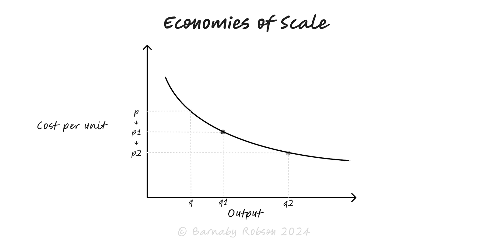
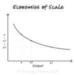
Economies of scale occur when average cost per unit falls as output rises. Fixed costs (plant, R&D, tooling, brand) are spread over more units; labour and machines specialise; suppliers give better terms; logistics densify. Beyond a point, diseconomies (coordination, complexity, congestion) can reverse the effect. Related but distinct ideas: economies of scope (shared inputs across products) and the experience/learning curve (cost drops with cumulative output).
Cost anatomy – Average cost at volume q: AC(q) = F/q + V(q), where F is fixed cost and V(q) is per-unit variable cost (which may also fall with scale).
Sources of scale
- Fixed-cost dilution – plant, software, compliance, marketing.
- Specialisation – narrower tasks, better tools, faster setups.
- Purchasing power – bulk discounts, better payment terms.
- Process + tech – automation, higher-throughput equipment, densified routes.
- Learning/experience – cost falls by x percent when cumulative output doubles (e.g., an 80 percent learning curve).
Shapes & thresholds – step-fixed costs create kinks (new line/shift); minimum efficient scale (MES) is where AC is near its floor.
External vs internal – industry-wide infrastructure or cluster effects (external) vs firm-specific advantages (internal).
Not the same as network effects – network effects raise value with users; scale economies lower cost with output.
Manufacturing & fulfilment – lines, changeovers, distribution density.
Software/SaaS – high fixed R&D, near-zero marginal cost; AC plunges with users.
Procurement – frame contracts, vendor consolidation, volume tiers.
Marketing – brand assets amortised over larger revenue.
Shared services – finance, support, data platforms amortised across business units.
Map the cost stack – split fixed vs variable; identify step-fixed thresholds (extra line/shift, licence tier, warehouse).
Plot AC vs volume – show current volume, MES estimate and step points; include capacity utilisation.
Quantify sources – price breaks, setup time cuts, automation gains, route density; estimate impact on AC and throughput.
Design the ramp – stage capacity (modular lines, cloud autoscaling), secure volume (contracts), and align funding.
Protect quality & lead time – standard work, buffers, maintenance, SPC; don’t trade pennies for defects.
Reinvest the wedge – pass some savings to win share, bank the rest to deepen the moat (automation, distribution).
Review periodically – costs, mix, and tech change MES; refresh the curve and thresholds.
Chasing scale without demand – stranded capacity and leverage risk.
Confusing scale with network effects – cheap units don’t guarantee adoption.
Diseconomies – coordination overhead, long queues, defect spikes at high utilisation.
Step shocks – a new plant raises F before volume arrives; model ramp and cash burn.
Mix drift – low-margin variants dilute gains.
Regulatory/antitrust – aggressive consolidation or pricing can trigger scrutiny.
Learning ≠ time – experience curve depends on cumulative output, not the calendar.