Probabilistic Thinking
Probability & decision science (Bayes, Laplace, de Finetti; modern forecasting and decision analysis)
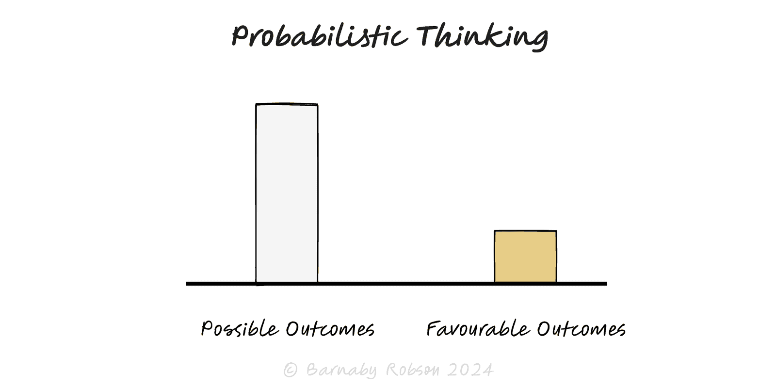
Probabilistic thinking treats the world as uncertain and quantifies that uncertainty. Instead of single answers, you work with distributions and odds; you compare options by expected value and risk of ruin; and you update beliefs when new data arrives (Bayes). It’s the antidote to wishful narratives and point-estimate plans.
Base rates (reference classes) – anchor beliefs to how similar cases actually turned out.
Expected value (EV) – for outcomes x_i with probabilities p_i: EV = Σ pᵢ·xᵢ. Use expected utility for large, risky stakes.
Distributions & tails – model the spread, not just the average; many domains are skewed or heavy-tailed.
Bayesian updating – Posterior ∝ Prior × Likelihood; make beliefs explicit and revise with evidence.
Dependence – check correlations; joint risks aren’t independent (conjunction/compound failures).
Value of information – buy tests/pilots only if EVPI/EVSI exceeds their cost and delay.
Aleatory vs epistemic – irreducible randomness vs uncertainty you can shrink with data.
Product bets (launch vs pilot), pricing and roadmaps.
Forecasts for demand, revenue, incidents and lead times.
Portfolio & capital allocation (position sizing, stop rules).
Operations & reliability (failure probabilities, capacity buffers).
Research & A/B tests (power, priors, decision thresholds).
Frame the decision – objective, horizon, unit (e.g., £, hours, risk points).
Write scenarios with probabilities – include downside. Example: 40% +£2.0m, 50% +£0.5m, 10% −£1.0m → EV = £0.95m.
Anchor to base rates – outcomes of similar teams/products; adjust for known deltas only.
Model the spread – list P50, P90, P99; use simple distributions (normal/lognormal) or a 10k-trial Monte Carlo for compound drivers.
Stress tails & ruin – if a path has non-trivial risk of ruin (cash to 0, legal loss, safety), cap exposure or redesign—even if EV is positive.
Plan updates – define what evidence will change your mind (metrics, dates) and by how much.
Decide with rules – go if EV clears hurdle and risk bounds hold; else pivot, stage, or kill.
Calibrate – record forecasts with probabilities; score with Brier/log scores; tighten over time.
Point estimates and “most likely” plans; communicate ranges and percentiles.
False precision – two decimals on weak inputs; show sensitivity and breakpoints.
Base-rate neglect – stories that ignore how similar cases usually end.
Independence assumptions – correlated bets fail together; check common shocks.
Mean worship – averages mislead in fat tails; manage percentiles and downside.
Positive-EV but ruinous – never trade solvency for EV; use limits and barbells.